Auto-regressive models

Auto-regressive models are a class of statistical models widely used in various fields, including natural language processing, time-series analysis, and image generation. These models predict a sequence of values based on previously observed values, making them well-suited for tasks that involve sequential data. Auto-regressive models have proven to be highly effective in generating realistic data and predicting future outcomes.

The history of the origin of Auto-regressive models and the first mention of it

The concept of auto-regression dates back to the early 20th century, with pioneering work done by the British statistician Yule in 1927. However, it was the work of mathematician Norbert Wiener in the 1940s that laid the foundation for modern auto-regressive models. Wiener’s research on stochastic processes and prediction laid the groundwork for the development of auto-regressive models as we know them today.

The term “auto-regressive” was first introduced in the field of economics by Ragnar Frisch in the late 1920s. Frisch used this term to describe a model that regresses a variable against its own lagged values, thereby capturing the dependence of a variable on its own past.

Detailed information about Auto-regressive models

Auto-regressive models are a subclass of time-series models where the value of a variable at a given time point is predicted based on its past values. In mathematical terms, an auto-regressive model of order “p” predicts the current value of a variable based on the “p” most recent observations.

The general form of an auto-regressive model of order “p” can be represented as follows:

Where:

• Y(t) is the value to be predicted at time “t.”
• Y(t-1), Y(t-2), …, Y(t-p) are the past values of the variable, up to order “p.”
• ε(t) represents the model’s error term, assumed to be white noise.

The order “p” determines how many past observations the model considers when making predictions. A higher order allows the model to capture more complex dependencies but may also lead to overfitting.

The internal structure of the Auto-regressive models – How Auto-regressive models work

Auto-regressive models are based on the assumption that the underlying data has a certain degree of temporal dependence. The model learns the relationships between past observations and the current value through a process called parameter estimation. The most common method used for parameter estimation in auto-regressive models is the method of least squares, which minimizes the sum of squared differences between the observed and predicted values.

Once the model is trained, it can be used for prediction by recursively generating future values. The auto-regressive nature of the model allows it to generate sequences of data points, making it particularly useful for tasks such as time-series forecasting, text generation, and music composition.

Analysis of the key features of Auto-regressive models

Auto-regressive models offer several key features that make them valuable for various applications:

1. Sequence Prediction: Auto-regressive models excel at predicting future values in a time-ordered sequence, making them ideal for time-series forecasting.
2. Generative Capabilities: These models can generate new data samples that resemble the training data, making them useful for data augmentation and creative tasks like text and image generation.
3. Flexibility: Auto-regressive models can accommodate different data types and are not limited to a specific domain, allowing their application in various fields.
4. Interpretability: The simplicity of the model’s structure allows for easy interpretation of its parameters and predictions.
5. Adaptability: Auto-regressive models can adapt to changing data patterns and incorporate new information over time.

Types of Auto-regressive models

Auto-regressive models come in various forms, each with its own specific characteristics. The main types of auto-regressive models include:

1. Moving Average Auto-regressive models (ARMA): Combines auto-regression and moving average components to account for both the present and past errors.
2. Auto-regressive Integrated Moving Average models (ARIMA): Extends ARMA by incorporating differencing to achieve stationarity in non-stationary time-series data.
3. Seasonal Auto-regressive Integrated Moving Average models (SARIMA): A seasonal version of ARIMA, suitable for time-series data with seasonal patterns.
4. Vector Auto-regressive models (VAR): A multivariate extension of auto-regressive models, used when multiple variables influence each other.
5. Long Short-Term Memory (LSTM) networks: A type of recurrent neural network that can capture long-range dependencies in sequential data, often used in natural language processing and speech recognition tasks.
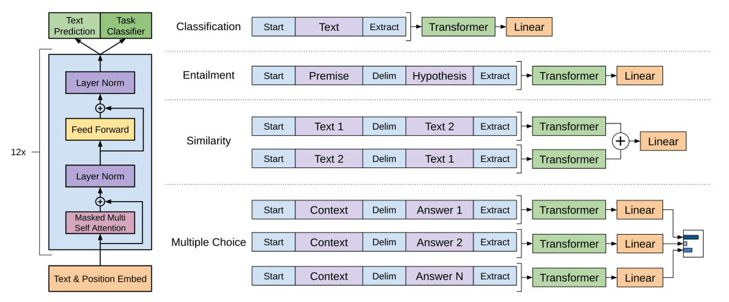
6. Transformer models: A type of neural network architecture that uses attention mechanisms to process sequential data, known for its success in language translation and text generation.

Here’s a comparison table summarizing the main characteristics of these auto-regressive models:

Ways to use Auto-regressive models, problems and their solutions related to the use

Auto-regressive models find applications in a wide range of fields:

1. Time-Series Forecasting: Predicting stock prices, weather patterns, or website traffic.
2. Natural Language Processing: Text generation, language translation, sentiment analysis.
3. Image Generation: Creating realistic images using Generative Adversarial Networks (GANs).
4. Music Composition: Generating new musical sequences and compositions.
5. Anomaly Detection: Identifying outliers in time-series data.

Despite their strengths, auto-regressive models do have some limitations:

1. Short-term Memory: They may struggle to capture long-range dependencies in data.
2. Overfitting: High-order auto-regressive models may overfit to noise in the data.
3. Data Stationarity: ARIMA-type models require stationary data, which can be challenging to achieve in practice.

To address these challenges, researchers have proposed various solutions:

1. Recurrent Neural Networks (RNNs): They provide better long-term memory capabilities.
2. Regularization Techniques: Used to prevent overfitting in high-order models.
3. Seasonal Differencing: For achieving data stationarity in seasonal data.
4. Attention Mechanisms: Improve long-range dependency handling in Transformer models.

Main characteristics and other comparisons with similar terms

Auto-regressive models are often compared with other time-series models, such as:

1. Moving Average (MA) models: Focus solely on the relationship between the present value and past errors, whereas auto-regressive models consider the past values of the variable.
2. Auto-regressive Moving Average (ARMA) models: Combine the auto-regressive and moving average components, offering a more comprehensive approach to modeling time-series data.
3. Auto-regressive Integrated Moving Average (ARIMA) models: Incorporate differencing to achieve stationarity in non-stationary time-series data.

Here’s a comparison table highlighting the main differences between these time-series models:

Perspectives and technologies of the future related to Auto-regressive models

Auto-regressive models continue to evolve, driven by advancements in deep learning and natural language processing. The future of auto-regressive models is likely to involve:

1. More Complex Architectures: Researchers will explore more intricate network structures and combinations of auto-regressive models with other architectures like Transformers and LSTMs.
2. Attention Mechanisms: Attention mechanisms will be refined to enhance long-range dependencies in sequential data.
3. Efficient Training: Efforts will be made to reduce the computational requirements for training large-scale auto-regressive models.
4. Unsupervised Learning: Auto-regressive models will be used for unsupervised learning tasks, such as anomaly detection and representation learning.

How proxy servers can be used or associated with Auto-regressive models

Proxy servers can play a significant role in improving the performance of auto-regressive models, particularly in certain applications:

1. Data Collection: When gathering training data for auto-regressive models, proxy servers can be used to anonymize and diversify data sources, ensuring a more comprehensive representation of the data distribution.
2. Data Augmentation: Proxy servers enable the generation of additional data points by accessing different online sources and simulating various user interactions, which helps in improving the model’s generalization.
3. Load Balancing: In large-scale applications, proxy servers can distribute the inference load across multiple servers, ensuring efficient and scalable deployment of auto-regressive models.
4. Privacy and Security: Proxy servers act as intermediaries between clients and servers, providing an additional layer of security and privacy for sensitive applications using auto-regressive models.

Related links

For more information on Auto-regressive models, you can explore the following resources:

1. Time Series Analysis: Forecasting and Control by George Box and Gwilym Jenkins
2. Long Short-Term Memory (LSTM) Networks
3. The Illustrated Transformer by Jay Alammar
4. An Introduction to Time Series Analysis and Forecasting in Python

Auto-regressive models have become a fundamental tool for various data-related tasks, enabling accurate predictions and realistic data generation. As research in this field progresses, we can expect even more advanced and efficient models to emerge, revolutionizing the way we handle sequential data in the future.